Lightware
Foci on the Lattice Flex, it's the rational abacus.
Key Advantages
- Consistency Across Scales: Every integer, whether large or small, is treated with equal computational weight in terms of amperage, allowing for streamlined energy usage.
- Immediate Fourier Transform Evaluation: The step increases in amperage are immediately ready for Fourier Transform analysis, avoiding the traditional delays caused by cycling through bit transformations, which can result in timing issues in other systems.
- Real-Time Data Handling: This system provides an efficient solution for real-time applications where high-frequency data or signals need fast and accurate processing without risking synchronization errors.
Applications
- Sensor Networks: Calibration of sensors distributed in 3D space can observe moving masses with certainty, leveraging scientific verification to ensure accuracy in measurements.
- High-Speed Communications: In environments requiring rapid processing, the elimination of bit transformation cycles significantly reduces latency, improving the system's responsiveness.
- Quantum & Physical Simulations: This approach is particularly valuable for simulations that need to handle large scales of data while maintaining energy efficiency and precise timing.
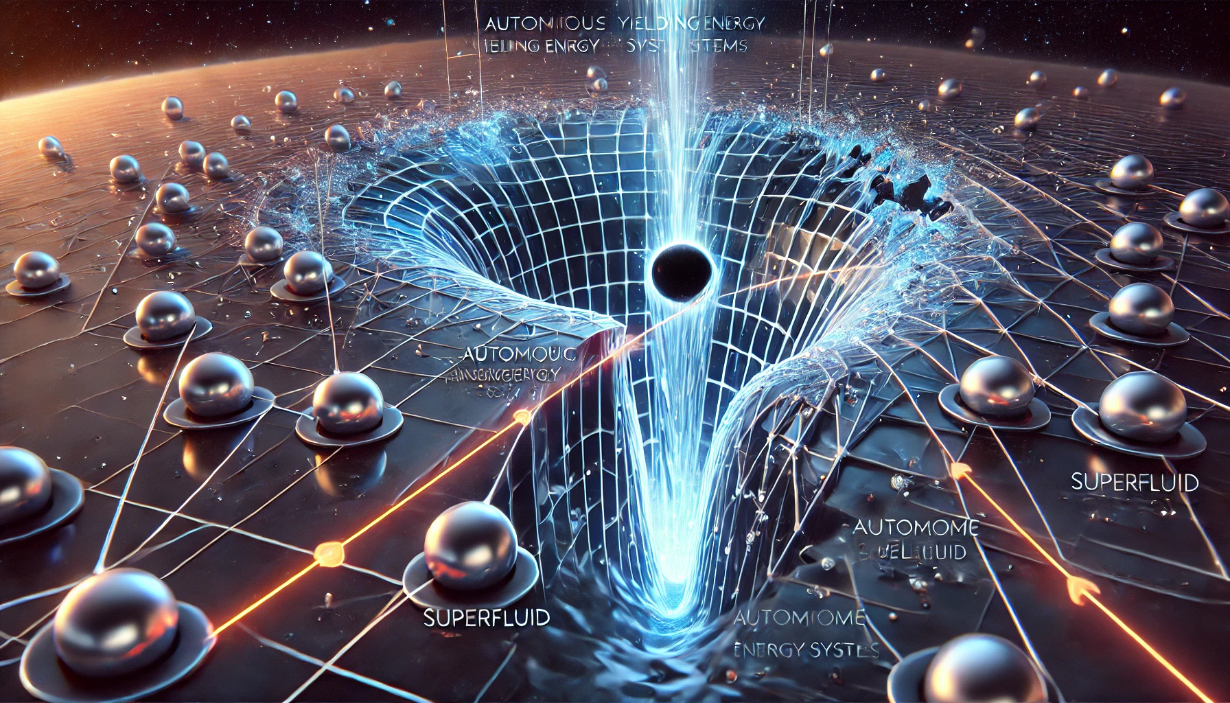
Introduction to the Spherical Matrix
At the heart of the Lightware system lies a groundbreaking concept: the Spherical Matrix. This matrix serves as a dynamic platform for processing optical data in three-dimensional space, redefining the way light is captured, analyzed, and redirected. With the ability to synchronize multiple light sources and wavelengths, it offers unparalleled control over optical phenomena.
Imagine light as not merely something that travels through space, but something that exists in a multi-layered 3D environment. The Spherical Matrix leverages this concept to handle the complexities of light in motion, allowing for data refinement in real time. It does so by comparing light data across spherical coordinates, effectively creating a system where optical flows are managed with near-perfect precision.
Optically Steering the Information Channel
The true power of the Spherical Matrix lies in its ability to steer optical information channels. Unlike traditional systems that process light in a linear manner, the Spherical Matrix uses a sophisticated system of polarized three-axis comparisons. These comparisons establish a triangular data channel that handles information along three distinct axes, each representing a specific dimension of 3D space.
This optical channel system creates a powerful dynamic where data can be continuously redirected based on real-time feedback. When spheres (representing internal and external optical layers) interact with incoming light, they create layers of data flow. This allows for the precise manipulation of light and optical properties in ways that are impossible with traditional flat-plane systems.
The Role of SLEDs in Data Distribution
At the core of the Spherical Matrix's efficiency are the Superluminescent Diodes (SLEDs), which serve as an example for data distribution and sensing. Positioned along the matrix's three primary axes, these diodes work to amplify, split, and distribute light data into three optical volumes.
The use of SLEDs enables the matrix to synchronize data across multiple wavelengths, ensuring that light is evenly distributed throughout the system. By applying orthogonal frequency division multiplexing (OFDM), the SLEDs split the incoming light into manageable parts, allowing the matrix to process it more efficiently.
Quantum Dots and Photoluminescence Routing
The system's routing capabilities are further enhanced by the inclusion of Quantum Dots (QDs), which introduce a layer of photoluminescent precision. These dots act like microscopic instruments, absorbing and emitting light at specific wavelengths to ensure that the spherical matrix routes light accurately.
Imagine each quantum dot as a finely-tuned element that allows the matrix to manage light wavelengths with incredible precision. These dots not only aid in data routing but also help create depth maps, similar to LiDAR systems, providing a detailed 3D representation of objects being observed.
Smoothing Curve of Optical Focus
As light passes through the spherical matrix, the system continuously refines and smooths the optical data. The matrix’s structure enables it to gradually hone in on the focal point of the object being observed, ensuring a high level of precision. This smoothing curve acts like a natural adjustment mechanism, where the system corrects and sharpens the light data in real time.
Think of this process as refining an image with ever-increasing resolution. By the time the light reaches its final destination within the matrix, it is perfectly calibrated, offering an unfiltered, high-resolution view of the object.
Photocell Distribution and Data Refinement
Light detection in the spherical matrix is handled by an array of finely tuned photocells. These photocells work together to cancel out noise and redundancy in the optical data, leaving only the most accurate signals for analysis. The system takes advantage of overlapping photocells, which subtract redundant data in a process akin to how significant figures are refined in a mathematical operation.
Each photocell processes light from a specific wavelength or direction, refining the data it captures. This process provides the matrix with high-resolution depth data, allowing it to build a complete picture of the observed object with three-ratio division output. By using three points of observation, the matrix ensures that every bit of optical data is verified for precision before final processing.
Perspective Matching and Optical Volume
Another key feature of the spherical matrix is its ability to match perspectives across multiple points of observation. This is particularly useful when observing moving objects or dealing with a rotating system. The spherical matrix can align its internal channels to dynamically adjust to changes in perspective, ensuring that optical data remains coherent.
Whether dealing with the volume density of light or the surface bandwidth of the sphere, the matrix provides a complete representation of the light entering the system. This unique ability to handle both volume and surface data gives the matrix an unparalleled advantage in optical precision.
Protocol Matching – Synchronizing Optical and Digital Systems
The Need for Protocol Matching
The spherical matrix system processes optical data with an unparalleled level of precision, but in order to fully realize its potential, it must interface with external systems. These systems—whether digital, optical, or mechanical—operate using different communication standards and protocols. Protocol matching ensures that the spherical matrix’s output is compatible with the inputs of other systems, allowing for seamless data transfer and integration.
In essence, protocol matching is the process of translating the language of light into a form that external systems can understand and work with. Whether it’s calibrating the spherical matrix to a remote sensing platform or ensuring that digital and optical data streams are synchronized, protocol matching is a critical step in maintaining the integrity of the data as it moves between systems.
Optical Protocol Translation
At the core of protocol matching is the process of optical protocol translation. The spherical matrix generates light-based data that is highly analog in nature, yet this data needs to be transmitted to digital systems for further processing and analysis. This is where the optical-to-digital bridge comes into play.
Optical protocol translation involves converting wavelength-based data into a format that can be read and interpreted by external systems. This process often relies on the polarization matching techniques introduced in Chapter 3, ensuring that the light waves remain coherent as they pass through different mediums. Additionally, the system must account for the frequency ranges of the receiving devices, ensuring that the light data is correctly encoded for transmission.
This translation allows the spherical matrix to communicate with a variety of systems, from LiDAR platforms to fiber-optic networks, without losing any of the fidelity of the original data. By matching the optical protocol to the specific needs of the receiving device, the system ensures that the data is received and processed correctly.
Real-Time Calibration for System Matching
One of the key challenges of protocol matching is ensuring that the system can calibrate in real-time. As the spherical matrix interacts with different systems, the optical data needs to be adjusted on the fly to account for variations in protocol standards. This real-time calibration is achieved through a combination of feedback loops and adaptive algorithms, which constantly monitor the data stream and make adjustments as needed.
For example, when the spherical matrix interfaces with a remote telescope array, the system may need to adjust its output to match the telescope’s specific wavelength sensitivities. Likewise, when communicating with a quantum computing platform, the matrix might need to synchronize its light data with the platform’s qubit processing protocols.
This dynamic calibration ensures that the data remains accurate and coherent across a wide range of systems, allowing the spherical matrix to function as a universal interface for optical data processing.
Matching Analog and Digital Signals
In addition to optical protocol translation, the system must also ensure that its analog signals are compatible with digital processing platforms. This involves converting the analog optical data—captured through the spherical matrix—into a digital format that can be analyzed by external systems.
This conversion is achieved through a process of signal encoding, where the optical data is broken down into discrete units that can be interpreted by digital systems. The challenge here is maintaining the resolution and fidelity of the original data, ensuring that no information is lost during the conversion process.
This is where protocol matching becomes critical. The system needs to match the sampling rate and bit-depth of the external digital system, ensuring that the optical data is converted into the highest possible resolution. By synchronizing the analog and digital signals, the spherical matrix ensures that the data is both accurate and high-fidelity, regardless of the platform it is transmitted to.
Error Correction and Data Integrity
Another important aspect of protocol matching is error correction. As light data moves through the spherical matrix and is transmitted to external systems, there is always a risk of data degradation or interference. This can be caused by environmental factors, signal noise, or mismatches between the protocols of the transmitting and receiving systems.
To mitigate this, the spherical matrix employs a variety of error correction techniques. These include redundancy checks, where multiple copies of the same data are sent to ensure that any corrupted information can be replaced by a backup, and parity matching, where the system uses mathematical algorithms to detect and correct errors in real-time.
By implementing robust error correction mechanisms, the system ensures that the data remains coherent and reliable, even in challenging transmission environments. This allows the spherical matrix to maintain the integrity of the optical data as it is transmitted to remote systems or stored for later analysis.
Future Applications of Protocol Matching
As optical and quantum computing systems evolve, the need for adaptive protocol matching will become even more critical. Future iterations of the spherical matrix may need to interface with autonomous systems, AI-driven platforms, or even space-based communication arrays. Each of these systems will have its own set of protocols and communication standards, and the spherical matrix must be able to adapt to these new challenges.
By building on the foundation of protocol matching, future versions of the system will be able to handle increasingly complex data streams and interface with a wider range of platforms. This will allow the spherical matrix to remain at the forefront of optical data processing, ensuring that it continues to provide high-resolution, accurate data across all systems and applications.

OFDM Lightspeed Channels
The Quantum Dot Bridge – Routing Light with Precision
Introduction to the Quantum Dot Bridge
In the spherical matrix system, quantum dots (QDs) serve as a critical bridge, connecting various optical components and ensuring that light is routed with precision. These tiny, semiconducting particles have the unique ability to absorb and emit light at specific wavelengths, making them essential for managing and controlling the flow of optical information within the matrix.
The quantum dot bridge forms a vital part of the system’s infrastructure, allowing light to pass through different stages of analysis, reflection, and calibration without losing coherence or quality. By tuning the QDs to specific wavelengths, the system can route light into designated channels, ensuring that each wavelength is processed according to the needs of the optical system.
Wavelength Control and Routing
At the core of the quantum dot bridge is its ability to control and route specific wavelengths of light. The spherical matrix requires light to be divided into separate optical streams, with each stream carrying information about different aspects of the observed object. For example, green and red wavelengths can be routed through different quantum dots, each responsible for analyzing a specific portion of the optical spectrum.
This routing capability is akin to the way a conductor leads an orchestra, ensuring that each section plays its part at the right moment. The QDs act as gatekeepers, directing the light with precision and ensuring that it reaches the correct location within the system. This process creates a coherent flow of information, where each wavelength is handled according to its unique properties.
Photoluminescence and Data Bridging
The quantum dot bridge relies on photoluminescence to manage the flow of light through the system. When light interacts with a quantum dot, it absorbs the light and then re-emits it at a different, often lower energy wavelength. This re-emission is critical for bridging data across different sections of the matrix.
By using photoluminescence, the quantum dot bridge ensures that light maintains its coherence as it passes from one part of the system to another. It’s similar to how fiber optic repeaters work in long-distance communications, boosting the signal to ensure that no data is lost during transmission. The QDs act as optical repeaters, ensuring that light remains strong and clear as it moves through the matrix.
Precision Tuning and Depth Mapping
The quantum dot bridge also plays a crucial role in depth mapping, as introduced in Chapter 1. By tuning the QDs to specific resonance frequencies, the system can create depth maps for the object being observed. Each quantum dot is responsible for analyzing a particular aspect of the light’s wavelength and intensity, which then contributes to a highly accurate depth map of the observed object.
This precision tuning allows the system to create a three-dimensional representation of the object, where each depth layer is mapped according to the wavelength of light. This depth map is not only used for observation but also for calibration within the matrix, ensuring that the entire system operates with the highest level of accuracy.
Bridging the Optical and Digital Domains
One of the most significant aspects of the quantum dot bridge is its ability to bridge the optical and digital domains. In a traditional system, light is either processed in its analog form or converted into a digital signal for further analysis. The quantum dot bridge allows for a seamless transition between these two domains, ensuring that the data remains coherent and accurate regardless of the format.
By managing light at the quantum level, the system can create a hybrid model where optical information is processed as both analog and digital data. This dual-processing capability allows for greater flexibility and precision in the system, as it can handle a wider range of data types and formats. The quantum dot bridge acts as the key to this dual-processing approach, ensuring that light is accurately managed regardless of its state.
This chapter sets the stage for deeper explorations into the SLED slices and polarized heals in Chapter 3, ensuring that readers understand the foundational role the quantum dot bridge plays in routing light and data with precision.
For more in-depth exploration of how these systems tie into broader applications, you can explore related sections:
- Cube Systems Material — Learn more about how the foundational principles of light and energy distribution apply to advanced cube systems.
<= Home (Splash)